Making Images and Using NetCDF Files with IDL

The lidarscan code is a set of functions and procedures in IDL used to retrieve information from BSCAN files and create images from them. This code is used by entering the appropriate commands in the IDL runtime environment. IDL must be installed on your work computer. Your IDL path must include the lidarscan, coyote, and catalyst codes (inlcuding their subdirectories).

Updating your IDL path from the IDL Workbench
Manually updating your IDL path on a Unix system (method #1)
Manually updating your IDL path on a Unix system (method #2)
Creating a basic image from the IDL command prompt (example)
Example explanation
Examples of vector image creation
SetProperty Options
PlotScan Options
Lidarscan GUI Menu Bar
Lidarscan GUI Text Boxes
Lidarscan GUI Options
Using ImageMagick to manipulate images
Resources

To update your IDL path from the IDL Workbench:

Go to Window > Preferences > IDL>Paths.
Select Insert, and add the directory containing the needed IDL code.

(You can place a checkmark next to a directory, indicating that IDL should also check any subdirectories in that directory. One method is to place all code used by IDL in one folder, and tell IDL to check the subdirectories of that folder.)

To manually update your IDL path on a Unix system (method #1):

Make an IDL startup file.
- If you have already used IDL on your computer, there is probably a folder in your home directory called '.idl'. If there is not, create one (do not forget the period at the beginning).
- Inside of your '.idl' folder, create a file called '.idlstartup'. The file '.idlstartup' is simply a text file without a '.txt' extension. You can create it any way you can create a text file.
- Within IDL, type the following:
  pref_set, 'IDL_STARTUP', 'path-to.idlstartup', /commit

Edit '.idlstartup' so that it adds the desired directories to IDL's path.
- Commands stored in '.idlstartup' will be executed when IDL starts.
- The command to append a directory to IDL's path is as follows:
  !PATH=!PATH+':'+Expand_Path('directory-path')
- The command can be modified to include all subdirectories by adding a '+' sign:
  !PATH=!PATH+':'+Expand_Path('+directory-path')

To manually update your IDL path on a Unix system (method #2):

Add the following command to your bash profile:
export IDL_PATH=$IDL_PATH:+'directory-path'

A profile file is a start-up file of a UNIX user, like the 'autoexec.bat' file of DOS. When a UNIX user tries to login into their account, the operating system executes a lot of system files to setup the user account before returning the prompt to the user. The profile file you want to edit is probably '.profile' in your home directory.

Example of how to create an image (without vectors) from the command prompt in IDL:

IDL> myScan = Obj_New('LidarScan', 'filename')
IDL> myScan -> SetProperty, outputdirectory = 'output-directory', output_prefix = "REAL_", LOW_RANGE_COLOR = 'black', HIGH_RANGE_COLOR = 'white'
IDL> myScan -> PlotScan, 0, XRANGE=[-2.5, 2.5], YRANGE=[-5, 0], CBRANGE=[24,39], OUTPUT='EPS', ASPECT=1.0, QUALITY=4, TEXTSCALE=1.2, /NOGUI, /NOFILTER

Example explanation:

Line 1:
This creates a LidarScan object called 'myScan'. ''filename'' specifies a BSCAN file that stores the information we will use. ''filename'' must be written in the following format: 'REAL.year-month-day_hour-minute-second.bscan'. This is an example of what it would look like: 'REAL.20150329_100112.bscan'. If you just want to use the filename without the directory it's in, you have to be in its directory when you start IDL. If you don't do this, you must write out the entire directory for ''filename''. To put BSCANS in your local directory, you must get them from the typhon server. To do this, log onto typhon using 'sftp' and your account information: 'sftp -P 4964 username@typhon'. Then go to '/bulk_storage/REAL_bscans/year-month/year-month-day', e.g., '/bulk_storage/REAL_bscans/200909/20090910'. The BSCANS are arranged by the dates that they were made. So if you have a particular date in mind, it's easy to find the right BSCANS. If you don't have a particular date in mind, you can simply navigate through the directories once you get to 'REAL_bscans'. After you get to the correct year, month, and day of the desired BSCANS, use the 'get' command to copy the desired BSCANS from typhon to your local directory: 'get filename', e.g., 'get REAL.20090910_143427.bscan'. If you want to 'get' all of the BSCANS from a particular day, use 'get *.bscan'.

Line 2:
This line calls the SetProperty procedure to set some properties in the LidarScan object. These properties, except for the output-directory, are all optional. But they can help the image come out better.

Line 3:
This line calls the PlotScan procedure. PlotScan will create an image of a specified scan, and it can either display that image on screen or save the image to a file. The first portion of the command 'PlotScan, 0', specifies which scan to use from the file we specified in Line 1 of the example. In this case, we will be plotting scan 0 from the file specified as ''filename''. Most, if not all, modern BSCAN files include only one scan. So 0 is the default scan number. The next three options specify the x-range, y-range, and color bar range of the plot. The low range color and high range color specified in Line 2 of the example are the colors that will be applied to any points that fall outside of the specified color bar range. The fourth option sets the output to an EPS (Encapsulated PostScript) file. The default is to display the output on screen. By default, PlotScan will plot filtered data. The /NOFILTER flag will cause it to plot unfiltered data.

Examples of vector image creation:

From a PPI scan, no subsampling:

oScan = Obj_New('LidarScan', 'C:\data\REAL.20070321_041224.bscan')

oScan -> PlotScan, 0, $
      ; Output='EPS', NoGUI=1, $
      ; XRange=[2,-2], YRange=[-2,-7], Aspect=[5./4], $
      Image_Intensity=0.5, $             ; (0..1)
      Vectors=[$
               {nCDFfile: 'C:\data\VECTORS.20070321_041224.nc', $
                locXY: ['cx','cy'], $
                vecUV: ['u','v'], $
                vecScale: 25.0, $ ; e.g.: 10 m/s (36 km/h) * 25.0 = 250 m on plot
                thick: 2, $             ; thickness of line used to outline arrow
                color: 0, $             ; color of arrow from colortable
                vectorColorTable: 3, $  ; colortable index, default: same as image
                data_location: 0, $     ; 0=tail, 1=center, 2=head
                head_angle: 30, $       ; Angle in degrees of arrowhead to shaft
                head_size: 1.0, $       ; 1=lines half shaft-length
                filter: ''}]

From an RHI scan, with subsampling:

oScan = Obj_New('LidarScan', 'C:\data\REAL.20070426_225115.bscan')

oScan -> PlotScan, 0, $
      ; Output='EPS', NoGUI=1, $
      ; XRange=[2,-2], YRange=[-2,-7], Aspect=[5./4], $
      Image_Intensity=0.5, $             ; (0..1)
      Vectors=[$
               {nCDFfile: 'C:\data\Pierre\REAL_RHI_20070426225115.motion.nc', $
                locXY: ['x','z'], $
                vecUV: ['u','w'], $
                vecScale: 25.0, $ ;e.g.: 10 m/s (36 km/h) * 25.0 = 250 m on plot
                thick: 2, $    ; thickness of line used to outline arrow
                color: 'x' , $
                vectorColorTable: 3, $ ; colortable index, default: same as image
                data_location: 1, $     ; 0=tail, 1=center, 2=head
                head_angle: 30, $       ; Angle in degrees of arrowhead to shaft
                head_size: 1, $       ; 1=lines half shaft-length
                Subsample: 20, $         ; Superseded by X_Subsample or Y_Subsample
               	; X_Subsample: 5, $ 
                ; Y_Subsample: 20, $ 
                filter: ['magnitude GT 1']}]

From a PPI scan (two compatible vector specifications, use array of structures):

oScan = Obj_New('LidarScan', 'C:\data\REAL.20070321_041224.bscan')

oScan -> PlotScan, 0, $
      ; Output='EPS', NoGUI=1, $
      ; XRange=[2,-2], YRange=[-2,-7], Aspect=[5./4], $
      Image_Intensity=0.5, $             ; (0..1)
      Vectors=[$
               {nCDFfile: 'C:\data\VECTORS.20070321_041224.nc', $
                locXY: ['cx','cy'], $
                vecUV: ['u','v'], $
                vecScale: 25.0, $ ; e.g.: 10 m/s (36 km/h) * 25.0 = 250 m on plot
                thick: 2, $             ; thickness of line used to outline arrow
                color: 0, $             ; color of arrow from colortable
                vectorColorTable: 3, $  ; colortable index, default: same as image
                data_location: 0, $     ; 0=tail, 1=center, 2=head
                head_angle: 30, $       ; Angle in degrees of arrowhead to shaft
                head_size: 1.0, $       ; 1=lines half shaft-length
                filter: ''}, $
               {nCDFfile: 'C:\data\VECTORS.20070321_042154.nc', $
                locXY: ['cx','cy'], $
                vecUV: ['u','v'], $
                vecScale: 25.0, $ ; e.g.: 10 m/s (36 km/h) * 25.0 = 250 m on plot
                thick: 2, $             ; thickness of line used to outline arrow
                color: 128, $           ; color of arrow from colortable
                vectorColorTable: 2, $  ; colortable index, default: same as image
                data_location: 0, $     ; 0=tail, 1=center, 2=head
                head_angle: 30, $       ; Angle in degrees of arrowhead to shaft
                head_size: 1.0, $       ; 1=lines half shaft-length
                filter: ''}]

PPI scan, two differing vector specifications (requires pointers):

oScan = Obj_New('LidarScan', 'C:\data\REAL.20070321_041224.bscan')

oScan -> PlotScan, 0, $
      ; Output='EPS', NoGUI=1, $
      ; XRange=[2,-2], YRange=[-2,-7], Aspect=[5./4], $
      Image_Intensity=0.5, $             ; (0..1)
      Vectors=[$
               Ptr_New( $ ; Use pointer if structures don't have identical field names and types 
               {nCDFfile: 'C:\data\VECTORS.20070321_041224.nc', $
                locXY: ['cx','cy'], $
                vecUV: ['u','v'], $
                vecScale: 25.0, $ ; e.g.: 10 m/s (36 km/h) * 25.0 = 250 m on plot
                thick: 2, $             ; thickness of line used to outline arrow
                color: 0, $             ; color of arrow from colortable
                vectorColorTable: 3, $  ; colortable index, default: same as image
                data_location: 0, $     ; 0=tail, 1=center, 2=head
                head_angle: 30, $       ; Angle in degrees of arrowhead to shaft
                head_size: 1.0, $       ; 1=lines half shaft-length
                filter: ''}), $
               Ptr_New( $
               {nCDFfile: 'C:\data\VECTORS.20070321_042154.nc', $
                locXY: ['cx','cy'], $
                vecUV: ['u','v'], $
                vecScale: 25.0, $ ; e.g.: 10 m/s (36 km/h) * 25.0 = 250 m on plot
                filter: ''})]

SetProperty Options:

COLORTABLE: Color table index number. Default: 13.

DATADIRECTORY: Name of data directory where BSCAN files are located.

FILENAME: Name of new REAL BSCAN file to parse and read. Alternatively, you could call the OpenFile method.

LOW_RANGE_COLOR: Name of low range color.

HIGH_RANGE_COLOR: Name of high range color.

OUTPUTDIRECTORY: Name of output directory where graphic output files are written. Default: same directory in which Lidarscan program is found.

OUTPUT_PREFIX: String prefix attached to output filename, e.g., prefix_XXXXX.jpg.

PLOT_ANNOTATION_COLOR: Name of color used for axes, axes labels, and color bar labels.

PLOT_BACKGROUND_COLOR: Name of background color.

PLOT_GRID_COLOR: Name of grid color.

PLOT_RANGE_COLOR: Name of optional range marker color. This marker is controlled with DRAWRANGE keyword in PlotScan.

RANGE_ANNOTATION_COLOR: Name of label color for optional range marker.

METADATA_COLOR: Name of metadata color located above plot (start time, scan type, etc.).

PlotScan Options:

XRANGE: Two element array describing minimum and maximum x-coordinates of plot. X-axis usually runs from east to west, with REAL located at x = 0.

YRANGE: Two element array describing minimum and maximum y-coordinates of plot. Y-axis usually runs from north to south, with REAL located at y = 0.

ASPECT: Set to aspect ratio (y/x) of plot, e.g., ASPECT = 6./4. Default: ISOTROPIC.

BEAMRANGE: Two-element array, giving minimum and maximum beam range to plot. Used to zoom into beam.

CBRANGE: Two-element array, giving minimum and maximum threshold/range of colorbar.

DEPOLARIZATION: Normally, plot is made of backscatter intensity. If DEPOLARIZATION is set, depolarization ratio is plotted instead.

DRAWRANGE: Draws beam range numbers on plot.

FILTER_LENGTH: If image is filtered, median filter of this length is applied. Default: 333.

IMAGE_INTENSITY: Value in range 0.0 to 1.0, indicating how prominently to render image, with lower values fading into background (e.g., to allow better view of vectors). 0 gives no image. Default: 1.0.

NOGRID: Suppresses drawing of plot grid.

NOFILTER: Plots unfiltered/raw data.

OUTPUT: Output file type desired: 'BMP', 'PNG', 'JPEG', 'TIFF', 'PS', or 'EPS'.

QUALITY: Rendering quality of plot. 1 - low, 2 - medium, 3 - high, 4 - highest. Default: 3. Lower quality rendering will render faster.

RESOLUTION: Two-element array that gives XSIZE and YSIZE of output image when OUTPUT keyword is set to 'BMP', 'PNG', 'JPEG', or 'TIFF'. Ignored otherwise. Default: size of current display window.

SCALE_FACTOR: Applies only to PostScript output. If you wish to reduce PostScript output size to 3/4 of its original size, set SCALE_FACTOR = 0.75. If you wish to double its size, set SCALE_FACTOR = 2.

SCANTIME: SCANTIME = 0 displays start time of scan (default). SCANTIME = 1 displays end time. SCANTIME = 2 displays both start and end times.

SUCCESS: Set to 1 if scan is successfully plotted. Set to 0 otherwise.

TEXTSCALE: Scale factor applied to all text around plot and colorbar. Default: 1.0.

VECTORS: Structure, array of structures, or (if structures would not have identical field layouts) array of pointers to structures, describing one or more vector fields to be drawn over image. Each structure provided may have one or more fields listed below (the VECTORS structure is passed to PlotNCDFVectors):

nCDFfile: String containing filename of nCDF file, e.g., 'C:\data\myFile.nc'.

locXY: Array of two strings giving names of nCDF file fields to use for data location coordinates on X-Y plot. Data values are assumed to be in meters. e.g., ['cx', 'cy'], or for vectors from RHI scan, ['cx', 'cz'].

vecUV: Array of two strings giving names of nCDF file fields to use for data vector values U and V on X-Y plot. Data values are assumed to be in meters per second (m/s or m s^-1). e.g., ['u', 'v'], or for vectors from an RHI scan, ['u', 'w'].

subsample: Scalar integer giving how many steps to take along X and Y values when choosing columns and rows of gridded data points to be plotted as vectors. Default: 1.

x_subsample: Scalar integer giving how many steps to take along X values when choosing columns of gridded data points to be plotted as vectors. Default: 1. Supersedes field 'subsample'.

y_subsample: Scalar integer giving how many steps to take along Y values when choosing rows of gridded data points to be plotted as vectors. Default: 1. Supersedes field 'subsample'.

sample_location: [x, y] position (in meters) of vector (from nCDF fields referred to in 'locXY') desired to be in subsampled set, e.g., tower location.

filter(*): String which contains IDL expression to be evaluated with values for each data location, using nCDF file field. Where expression evaluates to true, vectors will be displayed. Otherwise not. NOTE: all variables, constants, operators, and parentheses used must be separated from one another by at least one space. Default: '' (all points). e.g., 'cy LT -4', or 'azimuth GT 149 AND azimuth LT 209 AND range LT 5500 AND speed GT 2.5'.

vecScale: For given (u, v) value, length as shown on X-Y plot will be multiplied by this value to give actual vector length to plot. This can be considered as duration in seconds, and drawn vector will be distance that particle would travel in wind from data location in that length of time. Default: 1. e.g., 25, where 10 m/s (36 km/h) vector * 25.0 = 250 m on plot.

thick(*): One of two options to control thickness of plotted vector arrows (for window or raster file display, this is in pixels and is rounded to nearest integer; for PostScript, this is roughly in points, or 1/72 inch). Default: 1. Scalar value to use for all vectors, e.g., 2, or string giving name of nCDF file field to use for each vector. Note: range of values seen in this field are given thick values from 1 to 4. e.g., 'speed'.

color(*): One of three options to control color of plotted vector arrows (color values refer to colors 0 to 255 in color table specified by 'vectorColorTable'). Default: 0. Scalar value to use for all vectors, e.g., 0, or string giving color name to look up with FSC_Color. String giving name of nCDF file field to use for each vector. Note: range of values seen in this field are given color values from 0 to 255. e.g., 'speed'.

vectorColorTable: Scalar integer indicating one of IDL's built-in colortables to use for arrow coloring. Default: same colortable as used for image display.

data_location: Scalar integer indicating what part of arrow to place at precise data location: 0 = tail, 1 = center, 2 = head. Default: 0.

arrow_style: Scalar integer indicating style of arrow to draw: 0 = outline, 1 = filled, 2 = filled with outline. Default: 1 (filled).

arrow_thick: Scalar float indicating how thick arrow shafts should be. 1 = 1.0 point, 21 = as thick as arrow head (making "stake" shape).

head_angle(*): One of two options to control head angle of plotted vector arrows (between shaft and each arrowhead line, in degrees). Default: 30. Scalar value to use for all vectors, e.g., 30, or string giving name of nCDF file field to use for each vector. Note: range of values seen in this field are given angle values from 0 to 90. e.g., 'speed'.

head_indent: Floating-point value between -1 and +1 giving indentation of back of arrowhead along shaft. 0 = triangular shape, +1 = arrowhead that's just two lines, -1 = diamond shape. Default: 0.4.

head_proportional: 1 = size of arrowheads proportional to their magnitude. Default: 0, makes all arrowheads same size. NOTE: When head_proportional = 0, arrows are shaped as follows: ArrowheadLength = (DataPointSpacing(Min(x,y)) / 2) * head_size, ArrowheadWidth = ArrowheadLength * Sin(head_angle), ArrowShaftThickness = ArrowheadWidth * (arrow_thick/21). When head_proportional = 1, those rules give shape of arrow which has length DataPointSpacing(Min(x,y)), and for other lengths it is scaled from that shape.

head_size(*): One of two options to control size of plotted arrowheads. Default: 1. Scalar value to use for all vectors, e.g., 0.5, or string giving name of nCDF file field to use for each vector. Note: range of values seen in this field are given size values from 0 to 2. e.g., 'quality'.

arrow_outline_color: Used when Arrow_Style = 2. String giving color name to look up with FSC_Color.

missing_dots: Draws dots where magnitude is 0 or data missing.

legend_box_color: String giving name of color to use for legend box background. Default: plot_background_color.

Block_Thick = block_inThick: Thickness of lines around vector data blocks. Default: 0.

Block_Color = block_inColor: Color of lines around vector data blocks. Default: 'black'.

Block_LineStyle = block_inLineStyle: Linestyle to use for vector data blocks. Default: 0 (solid). 0 = Solid, 1 = Dotted, 2 = Dashed, 3 = Dash Dot, 4 = Dash Dot Dot, 5 = Long Dashes.

Block_Subsubsample = block_Subsubsample: After vectors are subsampled, how to subsample.

Block_X_Subsubsample = block_X_Subsubsample: To choose which vectors' data to show.

Block_Y_Subsubsample = block_Y_Subsubsample: Block extents for.

Block_X0X1Y0Y1 = block_X0X1Y0Y1: Vector of four strings giving data fields for X0, X1, Y0, Y1. For data blocks (e.g., ['x0','x1','y0','y1']).

Stream_Thick = stream_inThick: Thickness of streamlines. Default: 0.

Stream_Color = stream_inColor: Color of streamlines. Default: 'black'.

Stream_PSym = stream_inPSym: Plot symbol to use for points on streamlines.

Stream_SymSize = stream_inSymSize: Size of plot symbols on streamlines.

Stream_Subsample = stream_subsample: Superseded by Stream_X_Subsample or Stream_Y_Subsample.

Stream_X_Subsample = stream_x_subsample.

Stream_Y_Subsample = stream_y_subsample.

Stream_Integration = stream_Integration: Default - 0.

Stream_Tolerance = stream_Tolerance: Default - ?.

Stream_Max_Iterations = stream_Max_Iterations: Default - 200.

Stream_Max_Stepsize = stream_Max_Stepsize: Default - 1.0.

Stream_Uniform = stream_uniform: Default - 0.

Path_DeltaT = path_inDeltaT: Time between scans in set of files. Default: 30.

Path_Thick = path_inThick: Thickness of pathlines. Default: 0.

Path_Color = path_inColor: 'black'.

Path_PSym = path_inPSym: Plot symbol to use for points on pathlines.

Path_SymSize = path_inSymSize: Size of plot symbols on pathlines.

(All other Stream keywords for data handling apply to pathlines as well.)

(*) NOTE - computed fields may use any nCDF file field, or any of the following:
- 'range': (Sqrt(X^2 + Y^2))
- 'azimuth': 90-ATan(Y, X) in range: 0 (North, through East...) to 359.99...
- 'elevation': ATan(Y, X); in range: -179.99...to 180
- 'speed': Sqrt(U^2 + V^2)
- 'magnitude': Sqrt(U^2 + V^2)
- 'direction': 90-ATan(V, U) in range: 0 (North, through East...) to 359.99...

Note on how arrow proportions are calculated (sequence is important):
- ArrowHeadLength = (Min(SubsampledDataXYSpacing) / 2) * head_size
- ArrowHeadWidth = ArrowHeadLength * Sin(head_angle)
- ArrowShaftThickness = ArrowHeadWidth * (arrow_thick/21)
- ArrowLength = DataUV * vecScale

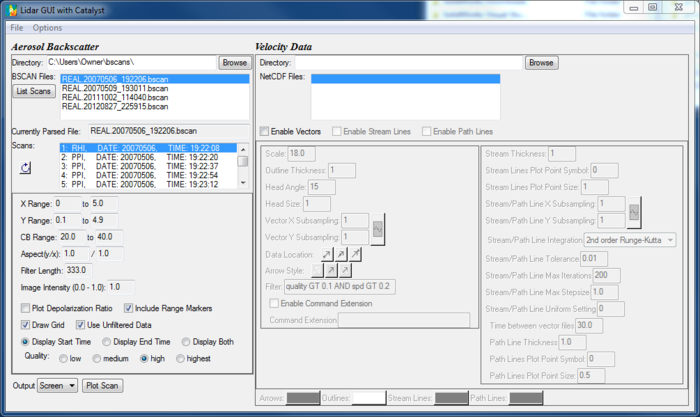
The Lidarscan GUI:

File > Load BSCAN: Opens dialog that allows you to select BSCAN file. Information will automatically be gathered from this file.

File > New Graphics Window: Creates new graphics window. If Output is set to 'Screen', IDL uses this graphics window to create plot. Allows you to create graphics window and resize it before clicking 'Plot Scan'. Can also be useful if you want to view multiple plots at once on screen.

File > Set Graphics Window: Sets which graphics window is active. IDL places plots in active window. Default = newest window. If you have created multiple graphics windows and want to change plot in older window, you must use this option. Active window is set by specifying an integer. You can see which integer corresponds to particular window in upper left corner of window.

File > Export Configuration: Saves options ('X Range', 'Y Range', 'Use Unfiltered Data', etc.) to file. Does not save vector options!

File > Import Configuration: Reads file saved with 'Export Configuration' and sets all options to values saved in file.

Options > Display Scan Info: Allows you to select which information is displayed in 'Scans' text box. Process of parsing older BSCAN files which contain large numbers of scans can take several minutes. Using this option to display fewer types of information can speed up parsing.

Options > Show Vector Parameters: Controls whether 'Velocity Data' portion of GUI is blank.

Lidarscan GUI Text Boxes:

Directory: Displays directory of currently selected file. Using 'Load BSCAN' to select file will fill this text box with directory of chosen file. 'Load BSCAN' option will also populate 'BSCAN Files' text box with any BSCAN files in same directory. You can use Browse button near 'Directory' text box to select directory instead of selecting particular file.

BSCAN Files: Lists all BSCAN files found in directory shown in 'Directory' text box. This text box will be populated after File > Load BSCAN is used to select file, or Browse button is used to select directory.

Currently Parsed File: Displays file that has been parsed. Scans in file are shown in 'Scans' text box.

Scans: Displays all scans within selected BSCAN file. There are three different types of scans which this may include: RHI, PPI, and stare. You must select the file type which you desire for your image. Selected BSCAN file is shown in 'Currently Parsed File' text box. 'Scans' text box will be automatically populated after File > Load BSCAN is used to select file. Small refresh button near this window can be used to re-parse currently selected file. Mostly useful if Options menu has been used to change information you want displayed about scans.

Lidarscan GUI Options:

X Range: Minimum and maximum values of x-axis.

Y Range: Minimum and maximum value of y-axis.

CB Range: Minimum and maximum values of color bar. Data points below minimum value displayed as color black, and points above maximum vlaue displayed as color white.

Aspect(y/x): Aspect ratio of plot. Describes lengths of x and y axes relative to each other. Does not affect range of values on x and y axes. Only stretches and compresses image. e.g., Aspect = 2 / 1 results in plot that is twice as tall as it is wide. For best results, make ratio between Y range and X range = aspect ratio.

Filter Length: Length of filter used when applying high pass median filtering to data.

Image Intensity: Controls image opacity. 1 = fully opaque. 0 = transparent. Only affects plot and color bar, not axes or labels.

Plot Depolarization Ratio: Check to generate plot of relative depolarization ratio instead of backscatter intensity. Depolarization ratio is ratio between backscatter intensities measured by two different channels on REAL.

Include Range Markers: Marks plot at radial intervals of two kilometers.

Draw Grid: Draws grid of dashed lines in between tick marks on axes. This is broken, and unchecking this will cause problems. Most forms of output will only produce solid black squares. The exception, eps output, will not include any labels.

Use Unfiltered Data: Displays data without applying high pass median filtering.

Display Start Time/Display End Time/Display Both: Controls what time to display at top of plot.

Quality: Controls plot quality.

Output: Controls where to put output when you press 'Plot Scan'. Includes image format of output file (e.g., EPS, PS, PNG, etc.). Default value of 'Screen' will draw plot in current active IDL graphics window. If no such window exists, one will be created. Other values for output allow you to save plot to different file formats.

Using ImageMagick to manipulate images:

ImageMagick is very useful for manipulating images made in IDL. Whether it be converting between file-types, or resizing for various purposes, it is a valuable tool to have handy. If you don't already have it installed on your computer, you can download the software for free from ImageMagick: Downloads. The installation instructions can be found at ImageMagick: Install from Source, and are fairly easy to follow.

ImageMagick is quite easy to use from the command line. Just go to the directory with the image(s) that you want to work with, and use ImageMagick commands from there. The two most important ImageMagick commands for working with IDL images are the command for converting between file-types, and the command for resizing images. The command for converting file-types is 'convert input-filename output-filename'. And the command for resizing images is: 'convert input-filename -resize output-image-dimensions output-filename'. (Note: it is often advantageous to make EPS or PS images in IDL to start with, because the resolution and overall quality are better than with PNG or JPEG images. Then you can use ImageMagick to convert from EPS or PS to PNG or JPEG. Usually, PNG is the desired file format.)

Convert file-type example:

convert 20070316222651.eps 20070316222651.png

Resize example:

convert 20070316222651.png -resize 200x200 20070316222651.png

Resources:

The UNIX School
UNIX Environment
Encapsulated PostScript
A brief introduction to the bash shell
IDL Workbench Guide
Raster (Bitmap) vs. Vector
IDL Tutorials
Comment (computer programming)
ImageMagick: Downloads
ImageMagick: Install from Source